Real-Time Anomaly Detection Using Multimodal Signals

What Is Real-Time Multimodal Anomaly Detection?

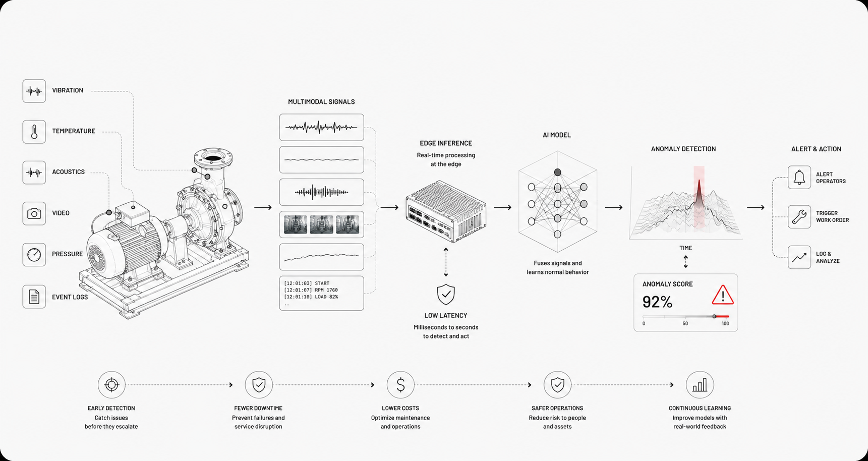
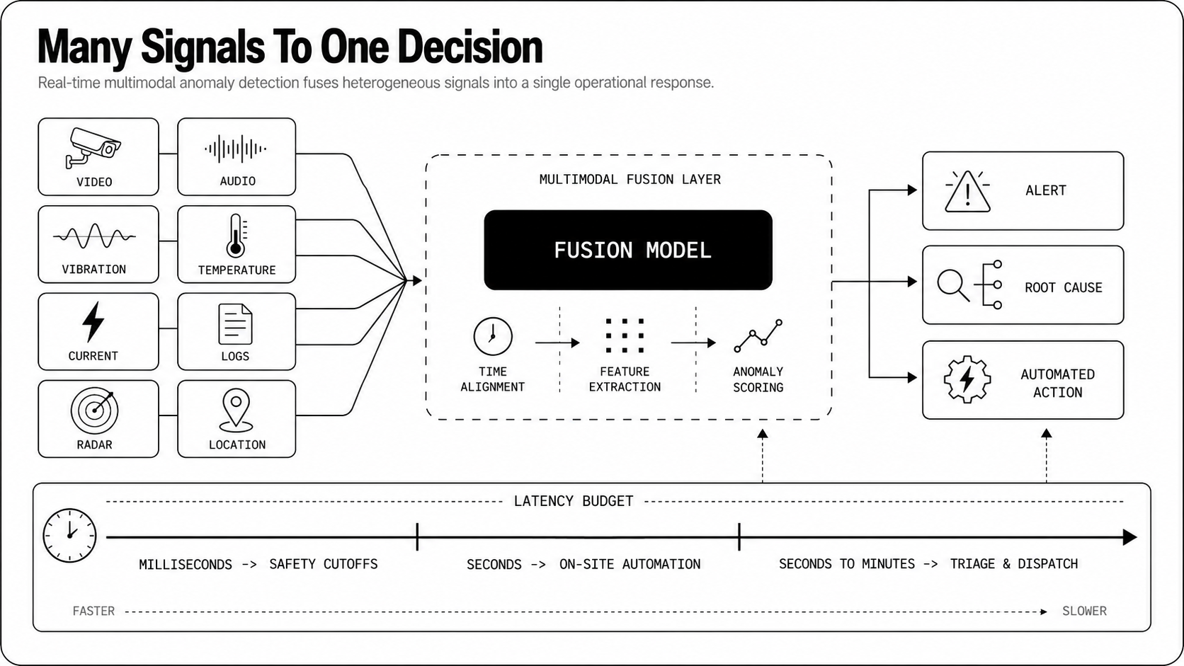
Real-time multimodal anomaly detection finds unexpected or harmful patterns by watching many kinds of signals simultaneously, and it does that with low enough delay to trigger actions while the event is happening. It’s not just spotting anything unusual, it’s spotting what matters for a defined operational response. The stakes are high: unplanned downtime now costs the world's 500 largest companies around $1.4 trillion a year, equivalent to 11% of their revenues, with an idle automotive line running to $2.3 million an hour, so catching the right event in time maps directly to uptime.

The physical world generates trillions of sensor signals that AI has barely touched, and this problem is about turning that raw volume into timely, reliable decisions. Physical AI — systems that perceive and reason about the physical world through sensor data — is becoming the foundation of industrial operations, and real-time anomaly detection is one of its clearest applications.

Define Objectives And Scope

Start by stating what counts as an anomaly for your business, who acts on alerts, and what outcomes follow. Is the goal operational safety, preventing downtime, reducing fraud, or prioritizing inspections? Decide whether detection triggers automated mitigation or human review. Define acceptable false positive and false negative rates, geographic and asset boundaries, and which modalities you’ll include. Scope keeps models focused, and it makes evaluation meaningful rather than vague.

Real-Time Constraints And Latency Targets

Set latency budgets by mapping detection-to-action timelines. Hard real-time cases need milliseconds to seconds, like collision avoidance or protective cutoffs. Soft real-time can tolerate seconds to minutes for triage or dispatch. Sampling rates, model complexity, and network hops determine feasible latency.

Place inexpensive preprocessing at the edge, where running anomaly detection cuts inference latency by an order of magnitude and buys more time to act, and reserve heavier inference in regional clouds if latency allows. Track throughput, CPU/GPU budgets, and SLA exposure, because delayed alerts are often as bad as missed alerts. Teams that standardize on Physical-AI infrastructure today build operational headroom they can extend asset by asset.

Why Fuse Multiple Modalities?

Relying on a single sensor type invites brittleness. Peer-reviewed work on industrial anomaly detection finds that methods built on a single data source can't fully exploit multimodal data, and that fusing modalities improves accuracy and stability when one signal is noisy or corrupted. Fusing signals uses the strengths of each modality to confirm, filter, and explain anomalies.

Just as large language models unlocked intelligence over text, foundation models are bringing that same leap to the physical world, and Physical AI extends that shift to real-world sensor data — and a foundation model like Newton, Archetype AI's model for the physical world, fuses hundreds of sensor types in one shared embedding space, so rare events that a single-signal tool would miss fall outside the learned geometry and reveal themselves.

Reduce False Alarms With Complementary Signals

Complementary signals act like cross-examination. A spike in vibration that coincides with a temperature rise looks more suspicious than either signal alone. Audio can confirm mechanical knocks that accelerometers suggest, camera frames can validate thermal hotspots, and logs can confirm operator actions.

Fusion reduces spurious alerts that come from sensor noise, maintenance activity, or transient environmental effects. This is the kind of distinction a foundation model makes natively: in a data center, Newton fused temperature with video to recognize that a temperature drop coincided with a person opening a door, telling a benign event apart from a true anomaly in a way single-signal monitoring cannot.

Improve Robustness Across Environments

Sensors fail or degrade with weather, lighting, interference, and occlusion. Multimodal systems keep working when one modality is compromised. Use radar when cameras see fog, thermal when visible light is low, and audio when visual occlusion occurs. This diversity handles domain shifts as systems move from lab to field, and it protects operations in diverse environments like construction sites, telecom sites, and smart city deployments.

Add Context For Root Cause Insight

Detection is only half the job, diagnosis closes the loop. Multimodal evidence narrows root cause hypotheses quickly. Time-aligned logs plus sensor patterns point to software regressions, hardware wear, or environmental triggers. Rich context shortens mean time to resolution and reduces wasted truck rolls. Engineers and operators can act with confidence when alerts carry corroborating signals, not just a single alarm flag.

Which Data Modalities Matter?

Pick modalities that give complementary views of the same event. Different domains favor different mixes, but a sensible baseline includes vision, acoustics, time series, textual metadata, and specialized sensors like radar or thermal.

Visual And Video Streams

Video captures shape, motion, and context. Use object detection, optical flow, and frame differencing to detect unusual movement, debris, or missing components. Video is high bandwidth and compute heavy, so extract compact embeddings at the edge. Privacy and storage policies matter, so consider selective retention and on-device anonymization.

Audio And Acoustic Sensors

Acoustic signatures reveal mechanical faults, impacts, and events invisible to cameras. Short-time Fourier transform features, spectral flux, and learned embeddings detect anomalies like bearing failure or gunshots. Microphone arrays add localization, which is useful for prioritizing inspections across a site.

Time Series Sensors And Logs

Vibration, temperature, current, pressure, and logs are the backbone of physical monitoring. They provide high-frequency, precise measurements for change point detection, trend analysis, and predictive models. Combine rolling statistics, frequency-domain features, and event markers to capture both sudden failures and slow degradation.

Text, Events, And Metadata

Maintenance notes, ticket histories, operator annotations, and system events add semantics that sensors lack. Natural language embeddings let you align human reports with sensor timelines. Text turns raw anomalies into actionable narratives, and it helps models learn which sensor patterns actually mattered historically.

Radar, Thermal, And Location Signals

Radar penetrates dust and smoke and measures motion robustly. Thermal highlights heat anomalies before visible effects appear. Location signals, including GPS and indoor positioning, tie events to assets and regions. These sensors shine in safety-critical, obscured, or dispersed deployments.

How To Preprocess Multimodal Streams?

Good preprocessing prevents garbage in and amplifies the value of fusion. It’s where operational constraints meet signal science.

Time Alignment And Resampling

Synchronize timelines with accurate timestamps, choose between NTP or PTP based on required precision. Resample signals to common timelines using interpolation or windowing when necessary. For event-driven streams, use temporal joins rather than fixed resampling. Misaligned modalities cause false mismatches and obscure causal links.

Denoising And Normalization Methods

Apply domain-appropriate filters, like bandpass for vibration, spectral subtraction for audio, and temporal smoothing for slow-changing sensors. Normalize per-device to remove unit and scale differences with z-score, min-max, or robust scaling based on median and IQR. Calibration drift must be monitored and corrected, because models learn device biases if you don’t.

Handling Missing Or Delayed Modalities

Design for partial observability. Use explicit masks so models know which modalities are present, apply statistical imputation for short gaps, and fallback rules for prolonged outages. Asynchronous architectures let late-arriving modalities augment or confirm earlier alerts instead of blocking detection. Graceful degradation, not brittle failure, wins in production.

Feature Extraction And Compression

Shift heavy feature extraction to the edge to lower bandwidth and latency. Convert raw signals into compact, informative representations: CNN embeddings for images, MFCCs for audio, spectral and wavelet features for vibration, and learned embeddings for text. Use dimensionality reduction like PCA, quantization, or lightweight autoencoders to compress while preserving anomaly information.

Foundation models for physical signals, like Newton, are pretrained self-supervised on hundreds of millions of real-world sensor measurements, so they supply reusable embeddings that cut custom engineering from scratch and speed deployment across sites — most use cases need no fine-tuning, just a handful of in-context examples.

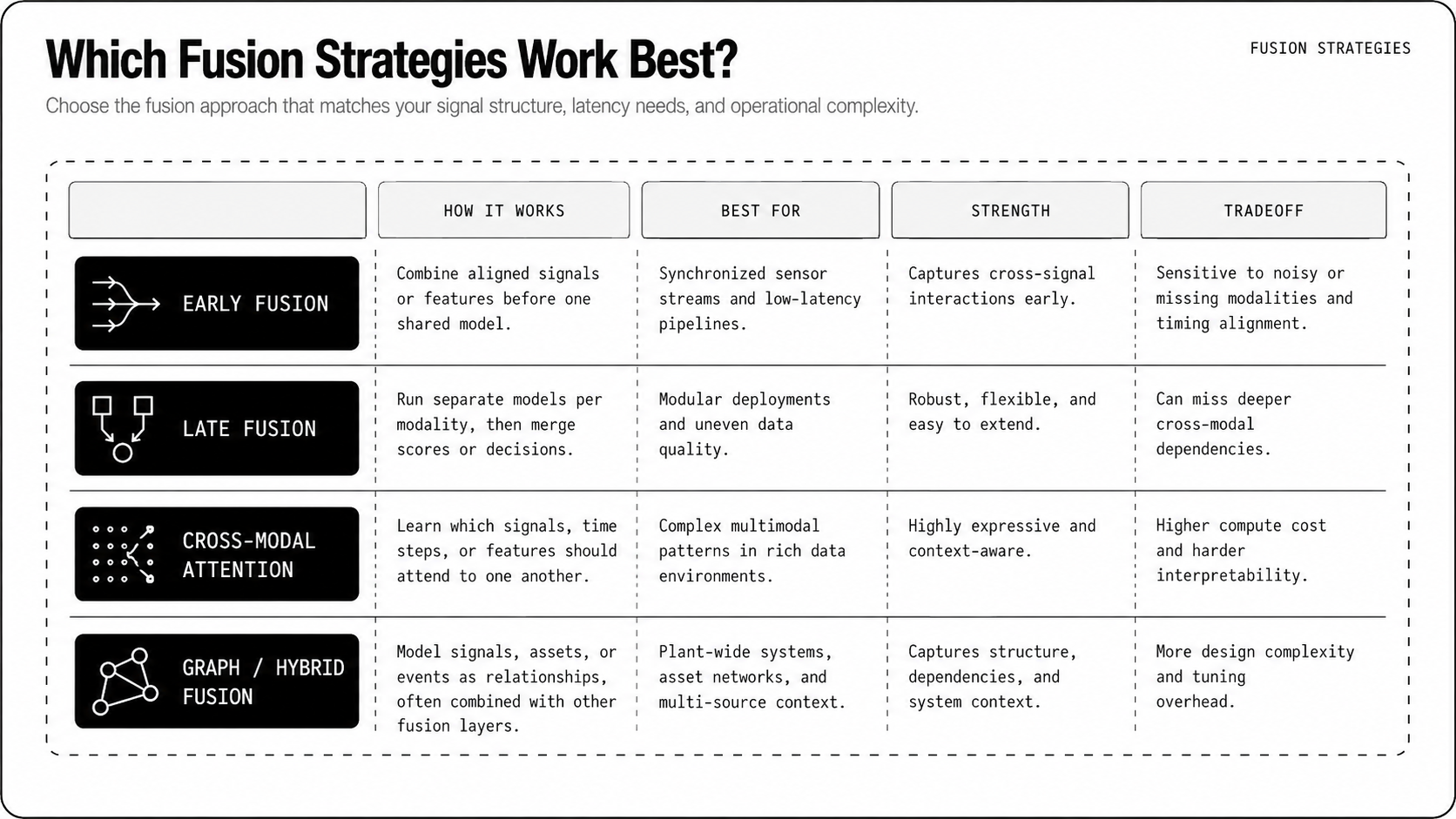
Which Fusion Strategies Work Best?

Early Fusion: Joint Representations

Early fusion projects each modality into a shared latent space and trains a single model on the concatenated representation. That approach captures fine-grained cross-modal correlations, so subtle combos of vibration, audio, and video produce stronger anomaly signals than any single stream. It needs careful time alignment and modality-specific encoders, and it struggles when a modality is missing or delayed. Use masks, modality-specific projection layers, and contrastive pretraining so the joint space stays meaningful across devices and domains.

For real-time systems, push heavy encoders to the edge and keep a compact joint head in the region or cloud. Physical AI platforms are the next step here: a foundation model like Newton, Archetype AI's model for the physical world, fuses hundreds of sensor types in one pretrained shared embedding space, so the fine-grained cross-modal correlations early fusion is after are already learned and reusable across assets, rather than rebuilt with modality-specific encoders for every new deployment.

Late Fusion: Ensemble Decisions

Late fusion keeps modality-specific detectors and merges their outputs at decision time, with voting, weighted averaging, or a meta-classifier. It’s robust to missing inputs, easier to interpret, and simpler to operate across teams and regulatory boundaries. The downside is lost opportunity to learn interactions that only appear when modalities are considered together. Late fusion works best when modalities have different latencies, privacy constraints, or compute footprints, and when you want graceful degradation rather than brittle joint models.

Cross-Modal Attention And Transformers

Cross-modal attention layers let one modality selectively focus on another, and transformers give you a unified architecture for temporal and spatial interactions. They excel when anomalies arise from complex, time-varying relations, for example audio cues aligning with brief visual occlusions. These models are data hungry and compute intensive, so use sparsity, causal masks, and distillation for production. You can also run cross-attention in two stages, cheap coarse attention at the edge and refined attention in the cloud, to hit latency targets.

Graph And Hybrid Fusion Approaches

Graph-based fusion models sensors and assets as nodes, edges encode spatial, physical, or causal relationships, and message passing propagates evidence across the network. They shine where topology matters, for example sensor grids across a construction site or a telco tower array. Hybrid solutions combine graphs with transformers or with late fusion ensembles, letting you capture local physical structure and global temporal interactions without a single monolithic model. Hybrid architectures are practical for teams building Physical AI infrastructure, because they map to operational layouts and scale predictably.

What Models Detect Anomalies In Real Time?

Lightweight Online And Streaming Models

Classic streaming methods like CUSUM, EWMA, incremental PCA, and streaming isolation forests run with bounded memory and constant update time. They’re ideal on the edge where milliseconds matter and compute is tight. Sketching, reservoir sampling, and approximate nearest neighbors let you summarize history cheaply. Implement them with rolling windows, decay factors, and explicit state checkpoints so models stay responsive while minimizing drift.

Deep Generative Models And Autoencoders

Autoencoders and variational models estimate normal behavior by reconstruction or likelihood, and anomalies are signaled by large reconstruction error or low probability. Conditional variants ingest multimodal context to avoid flagging benign deviations. Deep generative models capture complex, non-linear normal modes, but they can be slow and suffer from miscalibrated scores.

In practice, you can use pretrained embeddings from a foundation model and run a lightweight decoder at inference to get deep model power with lower latency. Newton, Archetype AI's foundation model for the physical world, is built for exactly this: pretrained self-supervised on hundreds of millions of real-world sensor measurements, it supplies reusable multimodal embeddings in which rare events fall outside the learned geometry and surface without explicit labels, so a lightweight anomaly head on top captures complex normal modes without training a deep generative model per asset.

Temporal Models: RNNs, TCNs, Transformers

RNNs and LSTMs maintain compact state and work well for modest sequence lengths, TCNs give parallelizable convolutional context with predictable latency, and transformers handle long-range dependencies and cross-modal attention. Choose RNNs or TCNs when you need consistent real-time throughput, pick transformers when interactions span long windows and you can afford more compute. Causal masking, state caching, and model distillation keep latency manageable in production.

Graph Neural Networks For Sensor Relations

Spatial-temporal GNNs model how anomalies propagate across physically related sensors, using dynamic graphs when topology changes. They detect collective or distributed anomalies that pointwise detectors miss, for example slow degradation spreading across a mechanical network. Localize computation by subgraph sampling and neighborhood caching to keep inference feasible on constrained hardware.

Scoring, Thresholding, And Calibration

Raw model outputs aren’t alerts until you score and threshold them. Use calibrated probability estimates where possible, apply Platt scaling or isotonic regression for classifiers, and model tails with extreme value theory for unsupervised scores. Dynamic thresholds per asset, seasonal baselines, and multi-window confirmation reduce flapping. Remember, lowering detection delay usually raises false positives, so tune thresholds to your operational cost function, not just a single metric.

How To Train With Limited Labels?

Self-Supervised And Contrastive Pretraining

Self-supervised tasks exploit structure in the streams: predict future frames, mask-and-reconstruct, align audio with video, or use temporal order discrimination. Contrastive losses that pull aligned multimodal chunks together and push misaligned ones apart create robust embeddings without labels. Those pretrained representations let you fine-tune tiny anomaly heads with very few labeled examples, which is exactly how teams scale across dozens of sites fast.

Synthetic Anomaly Injection Techniques

When real anomalies are rare, inject realistic faults into recordings or into a physics-based simulator. Perturb signals with realistic noise, change mechanical parameters, or synthesize occlusions in video. Domain randomization helps models generalize to unseen failure modes, but validate synthetic scenarios with operators so you don’t teach the model to chase unrealistic artifacts. Keep a mix of subtle and extreme injections so the detector learns both early warning signs and catastrophic events.

One-Class And Unsupervised Algorithms

One-class methods train on normal-only data, using deep SVDD, OC-SVM, clustering, or density estimation. They’re practical when anomalies are unknown or costly to label. These models need strong, stable features and continuous monitoring for concept drift, because normal behavior evolves. Combine several unsupervised detectors and use consensus or voting to improve robustness.

Active Learning And Human-in-Loop Strategies

Active learning targets scarce labeling budget where it moves the needle, for example uncertain alerts, rare clusters, or high-impact assets. Use uncertainty sampling, expected model-change, or operator-driven queues to get the right labels quickly. Human-in-the-loop systems do more than label, they provide weak signals like dismissals or corrective actions that feed back into thresholding and retraining. This is how teams bootstrap high-quality detectors without vast labeled corpora.

How To Evaluate Performance In Production?

Key Metrics: Precision, Recall, FPR, Latency

Precision and recall remain core, but in heavily imbalanced anomaly tasks precision often matters more operationally. Track false positive rate per asset and per time unit, not just global FPR. Measure end-to-end latency from event onset to actionable alert, because detection is useless if it’s too slow. Report resource metrics too, CPU, memory, and bandwidth, since those shape deployment feasibility. Production pipelines monitor both infrastructure and model-level metrics — throughput and resource use alongside prediction accuracy and anomaly scores — because either layer can be what fails.

Time-To-Detect And Detection Delay Metrics

Measure time-to-detect distributions, median and tail percentiles, and time-to-first-alert versus time-to-confirmation. For progressive events, use time-weighted miss penalties so late detection costs more. Set SLOs that reflect operational response windows, for example technicians arrive within X minutes after a confirmed alert.

Benchmark Datasets And Simulation Tests

Use replays of real multimodal streams and injected anomalies as benchmarks, and complement them with digital twin simulations to stress corner cases like correlated sensor failures or network outages. Reproducible replay tests let you compare models under identical timing and latency conditions. Track both aggregate scores and per-asset behavior, because a model that looks good on average can fail disastrously on a critical asset.

A/B Testing And Canary Deployment Methods

Validate model changes in shadow or canary mode before full rollout. Run the new detector in parallel and measure incremental detection, false alarms, and operator workload. Use phased rollouts with automated rollback criteria, and instrument human feedback as a metric in the experiment. Teams that treat model deployment like product rollouts, with monitoring, canaries, and automated retraining pipelines, will turn early Physical AI investments into durable operational advantage.

How To Deploy And Scale Systems?

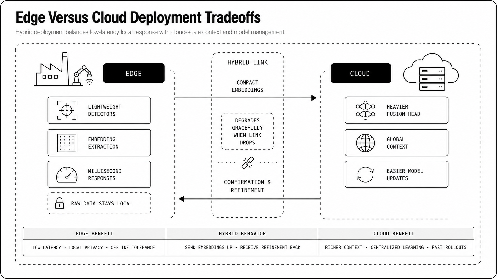
Edge Versus Cloud Deployment Tradeoffs

Edge inference reduces round-trip latency, keeps raw data local for privacy, and lowers bandwidth costs. Run fast, lightweight detectors or embedding extractors on the edge when you need millisecond to second responses. Cloud or regional inference gives you heavier models, global context, and easier model updates, but you pay network latency and higher egress.

Hybrid is the common sweet spot, an edge-cloud pattern with compact encoders at the edge and a richer fusion head in the cloud that confirms or refines alerts. Design around the worst-case network scenario so the system degrades gracefully, not catastrophically, when connectivity drops.

Physical AI platforms are the next step in resolving this tradeoff, because the same model can run wherever the workload needs it: Newton deploys in the cloud, in a customer's own VPC, or as a self-contained container on existing edge gateways down to hardware as modest as an Intel Atom, over MQTT and OPC UA, mirroring how most factory-floor Physical AI now runs on lightweight edge compute while keeping data residency with the operator.

Streaming Infrastructure And Protocols

Low-latency streaming is essential for early anomaly detection, because stale data leads to missed failure indicators, so design the transport for freshness. Choose protocols that match device constraints and latency needs: MQTT and CoAP for low-power telemetry, gRPC for efficient binary RPCs, and WebRTC or QUIC where peer streams and low jitter matter. Architect with append-only event logs so you can replay streams for debugging and testing. Partition by asset or site to keep hot paths small and cacheable. Use time-aware joins and watermarks for multimodal alignment, and keep side channels for metadata and operator notes so models get the context they need without stalling the main pipeline.

Model Optimization And Hardware Acceleration

Trim models with pruning, quantization, and distillation so they fit edge budgets without blowing up latency. Use operator fusion and fixed-point kernels to cut inference cost. On the hardware side, prefer accelerators designed for streaming workloads, like NPUs, edge GPUs, or small FPGAs, and match the model to the accelerator rather than forcing one to fit the other. Precompute heavy embeddings centrally when possible, and reuse foundation-model embeddings for multiple downstream detectors. Foundation models for physical signals, like Newton from Archetype AI, supply reusable representations that shrink per-site training and inference — and because one model ports across assets, extending a proven deployment from one machine to a fleet shifts from a per-asset project toward roughly same-week configuration, each new use case cheaper than the last.

Autoscaling, Fault Tolerance, And Rollback

Autoscale on meaningful signals, not raw concurrent connections, for example scale on active asset count or encoded throughput. Implement stateful checkpoints and idempotent processing so you can restart jobs without corrupting model state. Use canary or shadow deployments with automatic rollback triggers tied to false positive spikes, latency regressions, and operator feedback. Build circuit breakers and backpressure so downstream outages don't cascade into site-wide failures. Finally, keep runbooks and automated rollback scripts close, because for physical systems slow fixes are expensive.

What Operational Challenges Arise?

Concept Drift And Continuous Retraining

Physical systems change, sensors age, and environments evolve, so models drift. Detect drift by tracking feature distributions, embedding drift, and label shifts per asset. Automate retraining triggers that combine statistical drift signals with human review, and keep shadow models running to confirm improvements before rollout. Use rolling retrain windows, warm starts from foundation embeddings, and conservative validation on held-out, recent data to avoid catastrophic forgetting.

Managing Class Imbalance And False Positives

Anomalies are rare, and false positives cost attention and trust. Following the principle behind alarm rationalization, an alert that does not require a defined response should not exist, because nuisance alerts condition crews to tune out the system. Tune detectors to your operational cost function, not a single metric. Use cost-sensitive losses, resampling, focal loss, and synthetic injection to teach detectors subtle fault modes. Create hierarchical alerting, for example low-confidence notifications for human triage and high-confidence alerts that trigger automated mitigation. Track false positive rate per asset to spot brittle models fast, and include operator dismissal signals in active learning loops.

Privacy, Compliance, And Data Governance

Physical streams often carry sensitive information, especially video and audio. Minimize data collection and push anonymization to the edge, for example blur faces, strip identifiers, and retain embeddings instead of raw media when possible. Apply strong encryption in transit and at rest, enforce role-based access, maintain tamper-evident audit logs, and codify retention and deletion policies per jurisdiction. Compliance is not a checkbox, it’s an operational boundary that shapes architecture and determines which modalities you can legally deploy.

Explainability And Root Cause Analysis

Operators need actionable context, not opaque scores. Provide per-modal attribution so alerts show which signals contributed most, include short aligned timelines and representative frames or audio snippets, and surface likely root cause hypotheses with confidence levels. Use simple surrogate models or decomposed scoring alongside deep models to offer interpretable rationales. Build tools for quick causal tracing across sensors so humans can validate or disprove model hypotheses in minutes.

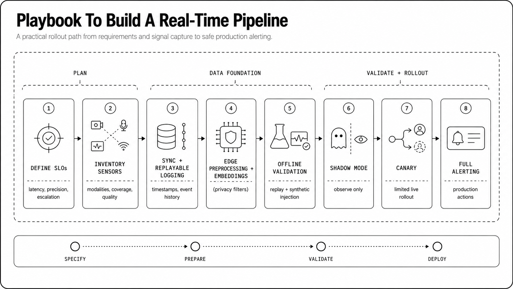
Playbook To Build A Real-Time Pipeline

Step By Step Implementation Checklist

• Define operational objective and SLOs, including latency, false positive cost, and response flows.
• Inventory sensors, sampling rates, and network topology.
• Implement time synchronization and stream replayable logging.
• Build edge preprocessors to extract compact embeddings and enforce privacy filters.
• Train and validate multimodal models offline with replay tests and synthetic injections.
• Deploy in shadow mode, run canaries, measure real-world precision and latency.
• Iterate thresholds, onboard operator feedback, and promote to full alerting progressively.

Monitoring, Alerting, And Incident Workflow

Monitor three axes: model health, data health, and system health. Track embedding drift, per-asset false positives, throughput, tail latency, and resource saturation. Alert on anomalies in model outputs and pipeline errors with tiered severity. Define incident runbooks: who acknowledges, who investigates, how to mute noisy alerts, and when to roll back. Use post-incident reviews to convert operational fixes into dataset improvements or feature changes.

Cost And Latency Budgeting Template

Allocate budgets across capture, edge compute, network, cloud inference, and storage. Start with a latency tree: sensor sampling to encoder, encoder to fusion, fusion to alert. Set hard SLOs for critical paths and soft targets for confirmatory signals. On cost, cap egress and cloud compute per asset class and prioritize expensive compute for high-value assets only. Recompute budgets when changing modalities or model complexity, and treat cost per alert as a primary metric for business tradeoffs.

Team Roles And Governance Model

Define clear ownership: device and edge code belong to site engineering, streaming and data ops own the pipeline, ML owns models and validation, SRE owns deployment reliability, and product owns objectives and ROI. Create a governance cadence with scheduled retrain approvals, quarterly drift reviews, and an escalation path for high-severity alerts. Give field teams simple feedback loops into labeling and synthetic scenario design so operational knowledge flows back into models. Teams building Physical AI infrastructure now will compound advantage as deployments scale.

How Does Multimodal Compare To Unimodal?

Performance Benefits Versus Added Complexity

Multimodal fusion improves robustness and reduces false alarms by cross-validating evidence across signals. It catches patterns that single modalities miss, especially when interactions matter. Run out of the box across 40+ sensors on complex wind turbines, Newton — Archetype's foundation model for Physical AI — surfaced nine previously unknown failure patterns that even industry experts had not catalogued, an estimated $50 million-plus in annual downtime impact, exactly the kind of multimodal insight a single-signal tool would miss. That gain comes with harder time alignment, more complex preprocessing, and larger testing matrices. Ask whether the improvement in detection and diagnosis justifies the engineering and operational cost for each asset class.

Maintenance And Operational Overhead

More modalities mean more sensors to calibrate, more drift surfaces, and more failure modes to monitor. Inventory and per-modality health metrics become essential. Maintenance cycles lengthen if you need coordinated firmware updates or cross-modal revalidation. You can reduce overhead by standardizing on shared embeddings and foundation-model primitives that multiple detectors reuse.

When To Choose Single Modality

Pick single modality when latency or cost is tight, when one sensor reliably captures the failure mode, or when privacy or regulation blocks other data types. Start unimodal to prove the detection concept quickly, then add modalities iteratively when you need higher precision or better root cause resolution. In many deployments, a pragmatic path is single modality for first-pass detection and multimodal confirmation for escalation, which balances speed, cost, and operational trust.

FAQs

Which Models Run Efficiently On Edge Devices?

Edge devices need bounded memory, predictable compute, and fast startup. Classic streaming algorithms, like CUSUM, EWMA, incremental PCA, and streaming isolation forests, are cheap and reliable for simple thresholds or change points. For learned models, prefer tiny CNNs, compact TCNs, distilled transformers with causal masking, and quantized LSTMs. Use pruning, quantization, and distillation to shrink larger architectures, and push heavy encoders offline or into regional nodes. Hardware-aware choices matter, pick models that map to NPUs, edge GPUs, or small FPGAs rather than forcing a one-size-fits-all design. Cache and carry state across windows, use operator fusion for common kernels, and reuse foundation-model embeddings where possible so the edge only runs a lightweight anomaly head. Foundation models for physical signals, like Newton, let you precompute reusable embeddings and avoid retraining full encoders per site.

How Do You Handle Missing Modalities At Runtime?

Design for partial observability from day one. Use explicit presence masks so models know which modalities are active. For short gaps, impute with statistical methods or replay recent embeddings; for longer outages, fall back to modality-specific detectors and raise degraded-confidence alerts. Late-fusion architectures or ensemble heads make graceful degradation easier, because decision logic still works with reduced inputs. Also treat late-arriving modalities as confirmatory evidence, not blockers, so initial alerts can be issued and refined when the missing stream returns. Train with simulated dropouts and modality-level noise so the model learns robust, conditional behavior. Finally, surface prolonged modality outages to operations as a first-class alert, because missing sensors often precede real incidents.

How Can I Reduce False Positive Rates?

Reduce false positives by requiring corroboration across time and modalities. Use per-asset, dynamic thresholds rather than a single global cutoff, and apply multi-window confirmation so a transient blip doesn't trigger an action. Calibrate scores with methods like Platt scaling or isotonic regression and model tail behavior with extreme value theory for unsupervised detectors. Ensemble different detectors and require consensus or weighted votes for high-cost actions. Incorporate contextual metadata, like maintenance windows and operator notes, to suppress known benign deviations. Feed operator dismissals back via active learning so the model learns what not to alert on. Finally, tier alerts: low-confidence notifications for human triage, high-confidence alerts that trigger automated mitigation, which preserves trust while keeping sensitivity high.

What Latency Is Acceptable For Real Time?

Latency depends on the action you want to enable. Milliseconds to low hundreds of milliseconds are needed for actuator-level, safety-critical interventions. Subsecond to a few seconds is typical for on-site automated responses and edge-based triage. Seconds to minutes suit dispatch, inspection scheduling, and human-in-the-loop workflows. Don’t pick a number in isolation, map detection latency to response timelines and cost of delay for your use case. Break end-to-end latency into capture, encode, transport, fusion, and decision steps and budget each segment. When lower latency raises false positives, use progressive confirmation: fast, low-confidence alerts followed by slower, high-confidence confirmation before costly actions.

Which Public Datasets Are Useful For Testing?

No single public corpus covers full multimodal industrial scenarios, but several datasets are useful building blocks:

• MVTec AD, for industrial image-level anomalies.
• DCASE and MIMII / ToyADMOS, for acoustic anomaly tasks and machine sound.
• Paderborn and NASA IMS bearing datasets, for vibration and rotating machinery faults.
• SWaT and WADI, for cyber-physical sensor networks in process control.
• SMD and Yahoo Webscope S5, for server and time-series anomaly benchmarks.
• NAB and the UCR archive, for diverse time-series change points and anomalies.These help validate model components, but expect to build replay datasets and synthetic injections for your exact multimodal stack. When public data is sparse, digital twins and carefully validated synthetic faults become essential for corner-case testing.

How Should I Label Anomalies For Training?

Label with operational purpose in mind, not purity. Choose label granularity that matches action: point-level timestamps for fast detection, window-level labels for progressive events, and event-level labels for incident resolution. Always tag severity and required response, and include modality availability and provenance so models can learn conditional behavior. Label maintenance windows, planned tests, and known benign anomalies explicitly to reduce noisy negatives. Use human-in-loop and active sampling to prioritize labeling of uncertain, high-impact cases. When you inject synthetic anomalies, keep provenance flags so training knows which examples are synthetic. Finally, maintain a held-out, recent test set per asset to detect overfitting and drift, and prefer conservative, high-precision labels for automated actions while using broader weak labels for triage models.

‍